We all know doing mathematical operations and functions is very easy in Microsoft excel. However, not all operations cannot be done very simply.
One such operation is calculating ratios. It requires two sets of formulas, however, still is efficient and very fast to calculate in excel.
There are mainly two ways by which you can calculate ratios in excel.
So, let’s learn how to calculate ratios in excel today.
What is Ratio?
Ratio displays a proportion. Essentially, it tells how much of one component there is relative to another component.
For example, if we say that Max has to mix 3 cups of flour with 2 cups of water to make a dough, the ratio of flour to water is 3:2.
To calculate this type of ratio, you can use two methods in excel.
The first one is the GCD method and the second one is with the TEXT and SUBSTITUTE formula.
So, let’s look at how to calculate ratios in excel.
How to Calculate Ratios in Excel?
A teacher wants to know the ratio of male and female students in the classes he teaches. So, first, he makes a table consisting of male and female numbers of students.
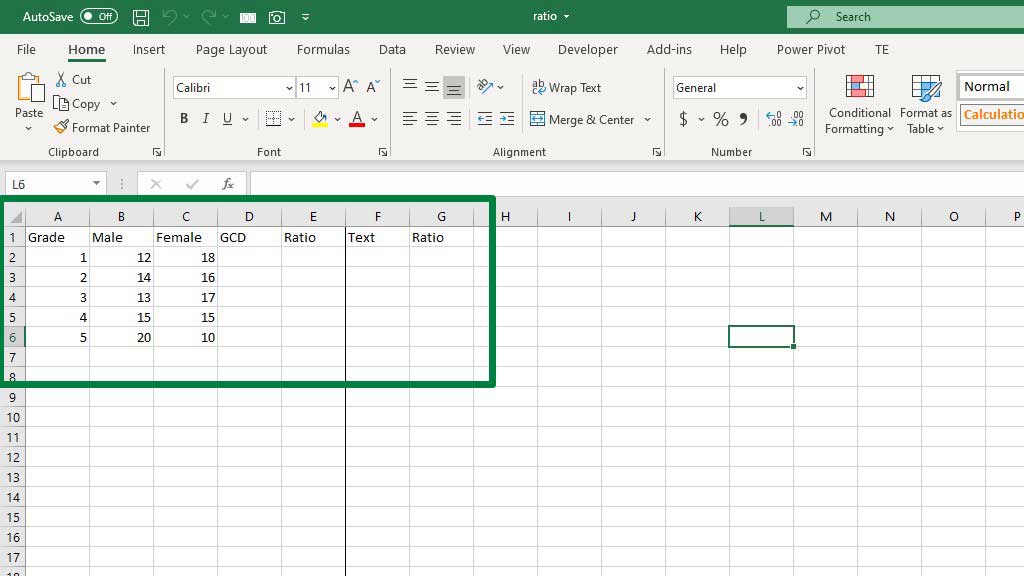
Now, time to calculate the ratio in excel.
Method#1 By calculating GCD
You need the GCD function in excel. GCD stands for the greatest common divisor. It basically finds out the largest number for both of the male and female students that will divide them equally without any remainder.
So, to calculate the GCD type the following formula:
=GCD(B2,C2)
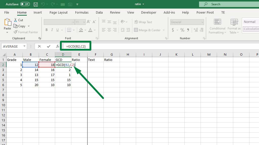
Then, drag the fill handle down to get the GCDs for all the grades or classes.
Now, the main hindrance of calculating a ratio in excel is if you divide the two components it won’t show you like the ratio format (a:b), it will show you as a decimal figure or you can use the text format to format it as a/b.
To solve this problem we are going to use & in excel to combine two numbers.
So, to get the ratio, type the following formula:
=B2/D2&”:”&C2/D2
Basically, divide the GCD by the first and second numbers consecutively and then combine the numbers with the help of &.
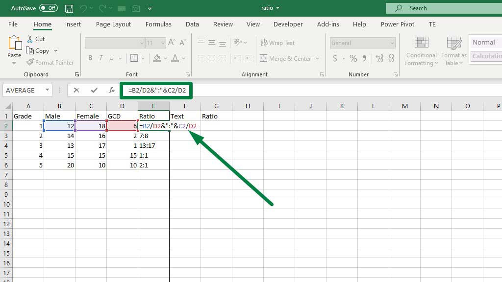
Drag the fill handle down to get the ratio for all of the classes.
Now, let’s see how to calculate ratio in excel by using the TEXT and SUBSTITUTE formulas.
Method#2 Using the TEXT and SUBSTITUTE formulas
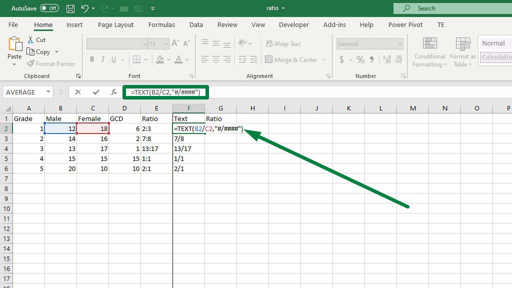
First, divide the first and second numbers and format them in this format “#/####”.
You can use the TEXT formula:
=TEXT(B2/C2,”#/####”)
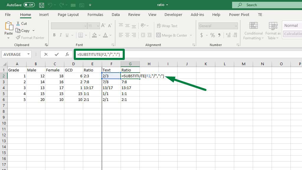
Now, simply if we can replace the oblique sign with a colon sign then we will get our ratios.
So, type the following formula to get the ratios:
=SUBSTITUTE(F2,”/”,”:”)
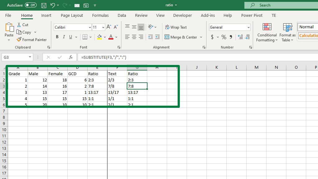
Basically, the substitute formula is used to replace the old text with new text. If you see the syntax of the formula:
=SUBSTITUTE (text, old_text, new_text, [instance]), you can see that first you have to select the existing text, then you have to type the text you want to replace, and finally, you have to type the new text you want to input.
Now, drag the fill handle down to get the ratios for all the classes.
=SUBSTITUTE(TEXT(B2/C2,”#/####”),”/”,”:”).
Conclusion
As I have said before, mathematical calculations are very easy in excel. Today you have seen another example.
Now, as you know how to calculate ratios in excel, you also can use this in long data sets where manual ratio calculations are almost impossible.

Hi there, I am Naimuz Saadat. I am an undergrad studying finance and banking. My academic and professional aspects have led me to revere Microsoft Excel. So, I am here to create a community that respects and loves Microsoft Excel. The community will be fun, helpful, and respectful and will nurture individuals into great excel enthusiasts.