How to Create a Bubble Chart in Excel?

In previous blogs, we have seen many graphs and charts in excel. For instance, the Venn diagram, burndown chart, supply and demand graph, stem and leaf plot, etc.

Some graphs have built-in features in excel, some are dynamic, some are not. However, the ability to use different types of graphs and charts in excel is very useful when it comes to visualizing data.

Among many graphs and charts that can be created in excel, the Bubble chart is certainly one of the most used ones.

It is visually appealing and distinguishable, and it helps identify multiple data points in a single graph.

So, let’s see how to create a bubble chart in excel.

Why Use a Bubble Chart?

Unlike column or bar charts, bubble charts can show individual data points. It also can show multiple values and labels in one graph.

It is essentially a bigger version of a scatter plot, so bubbles can be assigned different colors to make them distinguishable.

However, sometimes bubbles can get overlapped that can cause a bit of a problem.

But the use of bubble charts in displaying certain noticeable characteristics is very helpful.

So, let’s see how to create a bubble chart in excel.

How to Create a Bubble Chart in Excel?

The bubble chart is a built-in feature in excel. It is in the X Y (Scatter) charts section.

Let’s say you have three stocks of companies A, B, and C with their opening, closing price, percentage changes, and basis points.

You have to show the investors which stock is doing the best. In this scenario, you can use a bubble chart.

Follow the steps to create a bubble chart in excel.

Step#1 Create the Data Table

First, create a data table as shown in the picture.

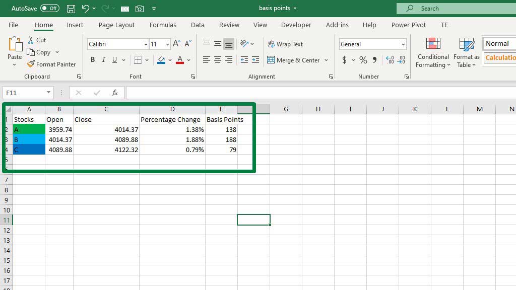
The color of the cell in column A represents the color of companies A, B, and C.

Step#2 Create the Data Table

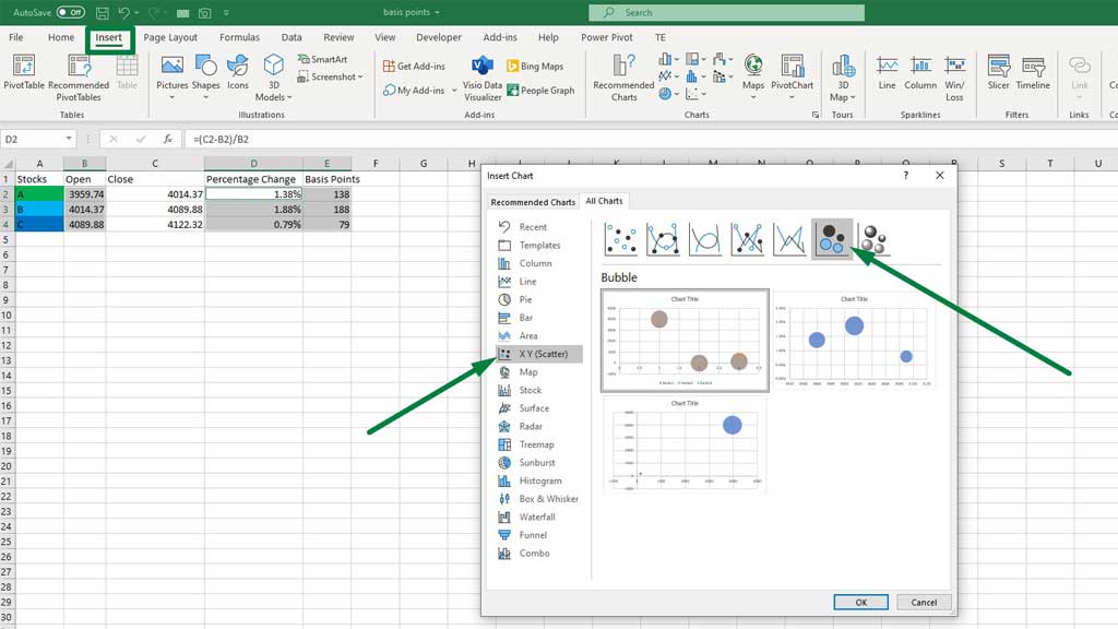
Select the opening prices column. Then holding the CTRL key select the percentage changes and basis points column.

Now, from the Insert ribbon go to Recommended Charts, and from the X Y (Scatter) select a bubble chart.

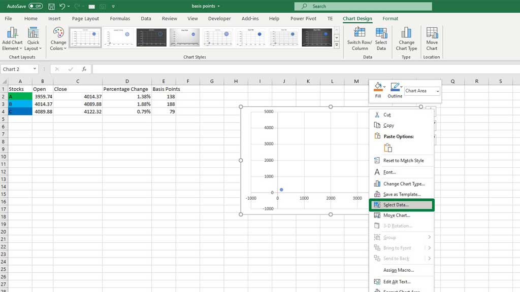
Step#3 Formatting the Data Series

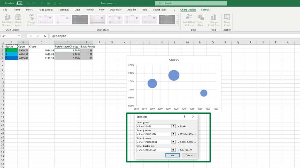
Right-click on the graph and go to Select Data.

You will see a dialogue box pop up. From that box go to Edit.

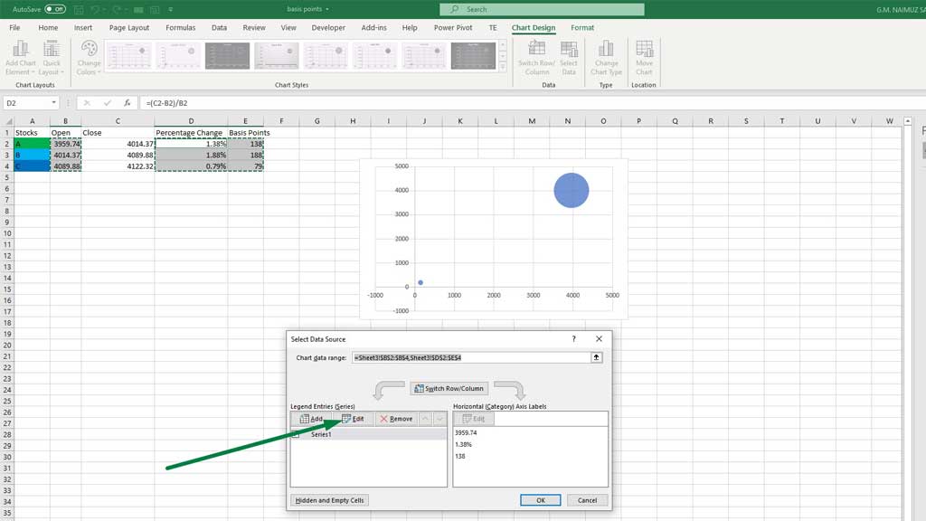
You will again see a dialogue box pop up. For series name assign Stocks. For series X values assign the column with the opening price, For Series Y values assign the column with the percentage changes, and finally for bubble size assign the column with basis points.

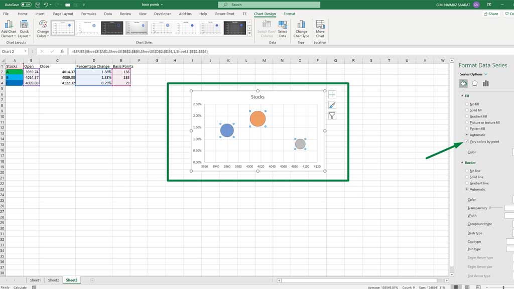
Now, click one of the bubbles, and enable the option Vary colors by point.

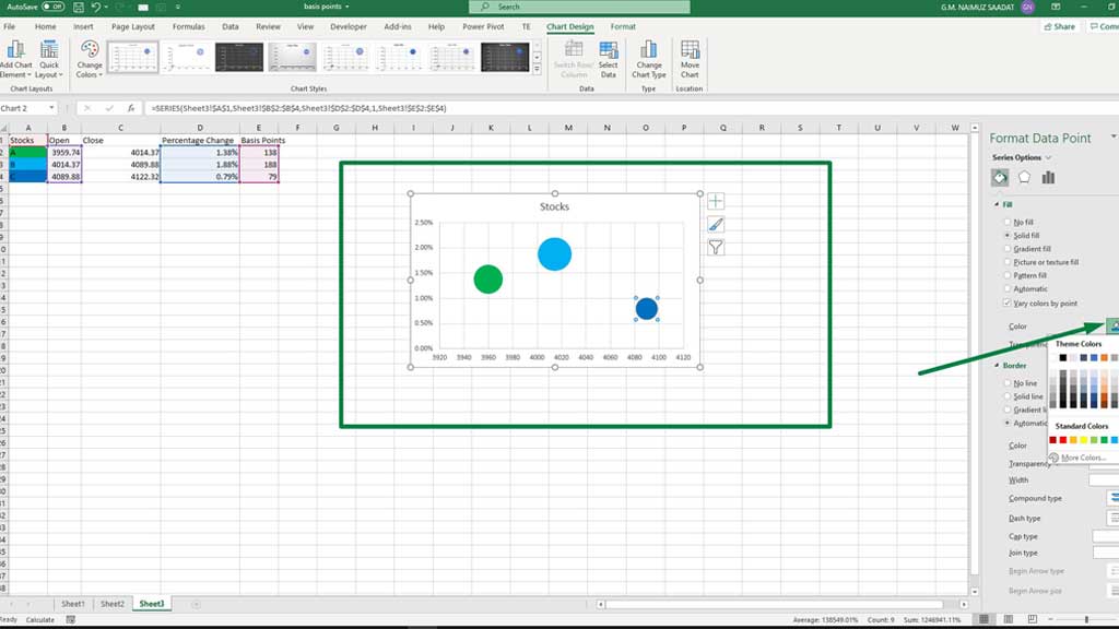
You can also choose your own color. For this case, let’s change the bubbles’ colors to the company colors from the color option.

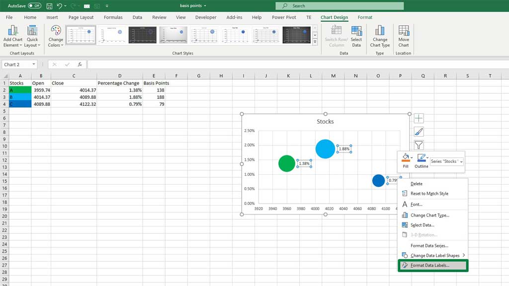
Now, click on one of the bubbles and right-click, and then enable data labels.

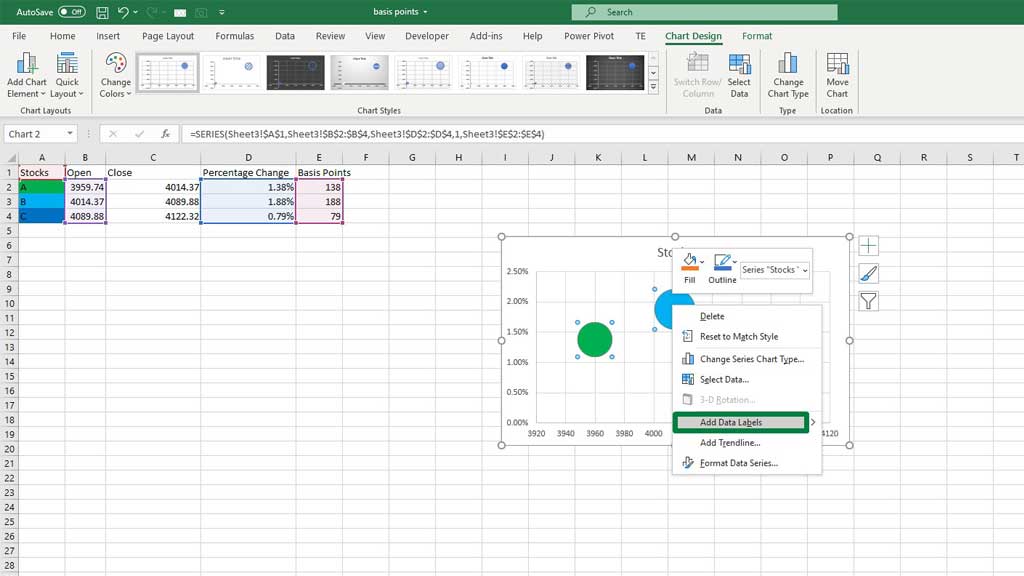
You can also format data labels, by right-clicking on one of the labels and going to format data labels.

There you go, your bubble chart in excel is ready. You can see that each stock’s characteristics are different, you can distinguish it and tell which bubble is bigger. A bigger bubble means better stock.

Conclusion

The bubble chart in excel is really useful to distinguish different characteristics of a data point. You can use it to make the audience connect with the data.

So, there you go, now you know how to create a bubble chart in excel.