
A good manager knows everything about the project he manages. A manager should be able to tell what the project is about, who are the team members, what’s the work progress, how much time it will take to finish the project etc.
A manager’s job is not easy, keeping track of all this information is very difficult. The job becomes even more difficult with the communication he has to maintain with clients and team members.
But there are some tools he can use to make his life easier, faster, and more efficient. One such tool is a burndown chart.
Let’s look at the process of how to create a burndown chart in excel.
What is a Burndown Chart?
A burndown chart simply means the chart that shows the burndown rate over a period. It is a mechanism that tracks progress and backlogs.
Imagine a code sprint. A manager is going to supervise a code sprint. The team consists of 3 developers and they have 7 days to finish the work.
So, let’s see how the manager can create a burndown chart in excel to keep track of all the activities.
How to Create a Burndown Chart in Excel?
To create a burndown chart in excel, there are some steps involved.
So, let’s get started on the steps on how to create a burndown chart in excel.
Step#1 Basic Information of the Sprint and Productivity level of the Workforce
This step is the foundation of any project. It includes the timings, workforce, and productivity levels.
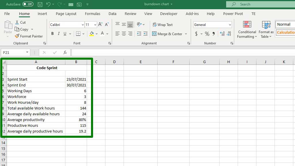
First, mention the sprint start date. In excel there is a shortcut to bring out today’s date, CTRL+;.
Then, use this formula:
to specify the end date for the sprint.
Then, as per company policy, specify the workforce size, working days, and total work hours per day.
To calculate the total available work hours, input this calculation:
Basically, multiply working days, workforce, and work hours per day to get the total available work hours.
To get the average daily available hours, divide “total available hours” by “total working days.” In excel, use the formula:
I have assumed the average productivity of 80% of the total available work hours. So, the productive hours’ formula is :
Lastly, the average daily productive hours can be calculated by dividing productive hours by working days. The formula is:
Step#2 Setting Up the Burndown Table
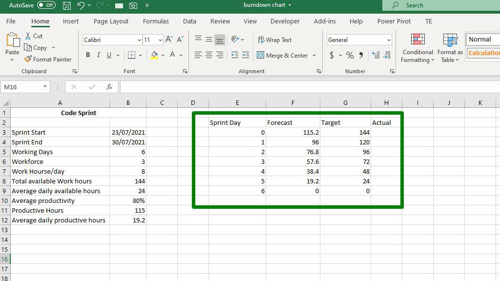
To set up a burndown table, you need four elements or columns. The columns are- sprint day, forecast, target, and actual.
Sprint day specifies the day of the sprint. It totals to the 6 working days available.
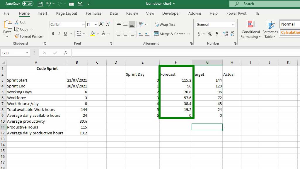
To get the forecast data, use the formula
The forecast is basically subtracting available daily productive hours based on the sprint day from the total available productive hours.
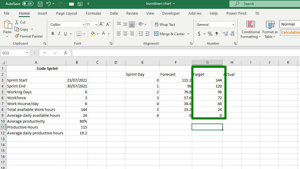
On the other hand, the target is the optimum level of effort. You can get it by subtracting available average daily hours based on the sprint day from the total available hours. Use the formula:
Actual is the real-time working hours based on how many people are working and how many hours of effort they have actually put in.
To calculate that, we need to set up a log table for the developers.
Step#3 Setting Up the Log Table
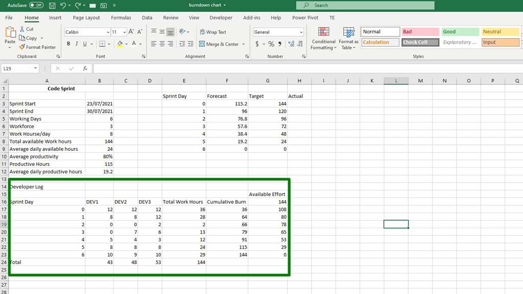
The log table contains the sprint day, one column for each developer or worker, total work hours, cumulative burn, and available effort.
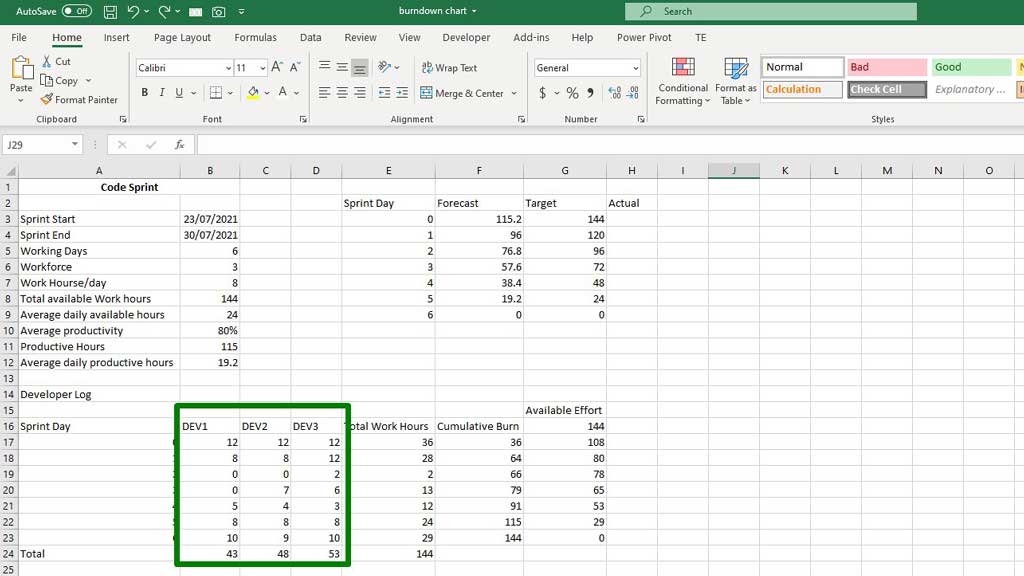
You can tell the developers to log their work hours daily in that table. You can see that each developer works at his/her own speed.
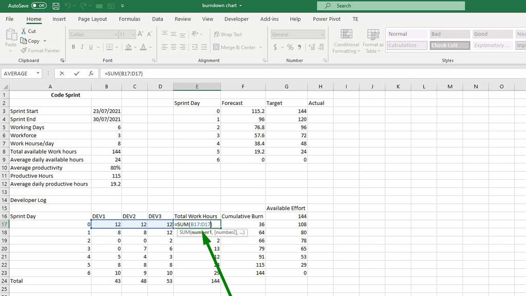
Total work hours is the sum of all the developers’ work hours for each day. You can use the SUM formula to calculate the total work hours. The formula is
Then drag the fill handle down to sum the other sprint days’ total work hours.
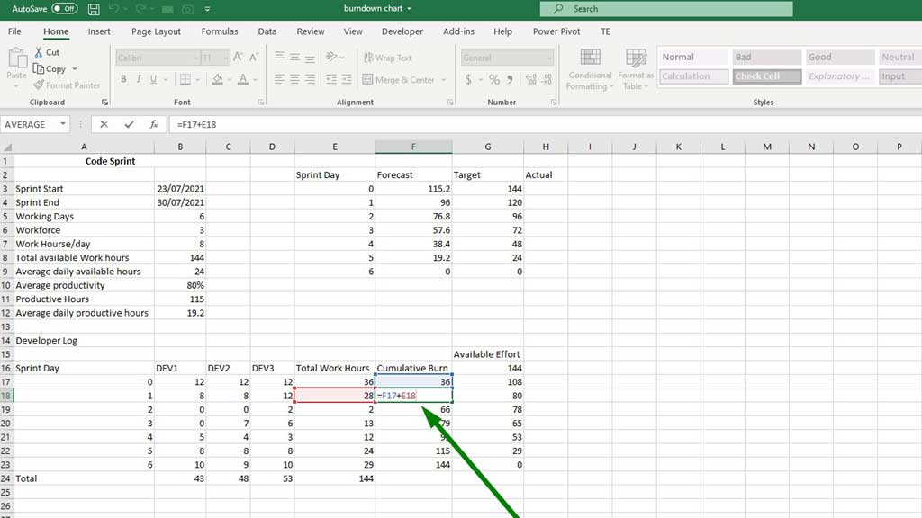
Cumulative burn is similar to calculating the cumulative frequency. The first cumulative burn is always equal to the first total work hours. Then use the formula
to calculate the second cumulative burn and drag the fill handle down to fill up the rest of the cumulative burns.
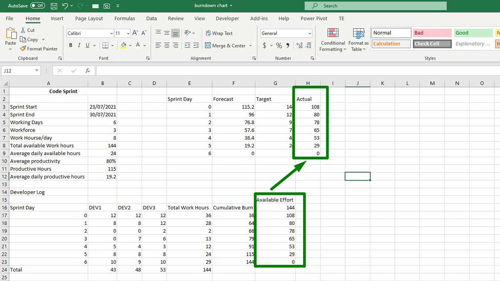
Step#4 Inputting the Actual Work Hours in the Burndown Table
The available effort calculated in step 3 is the actual hours. Input the data in the Burndown table and you are ready to create a burndown chart in excel.
Step#5 Create a Burndown Chart in Excel
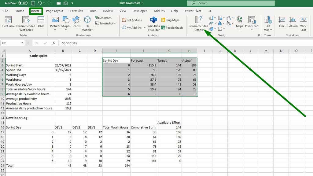
First, select the sprint day, forecast, target, and actual columns and go to the “Insert” ribbon and select “Recommended Charts.”
A dialogue box will appear from where you have to select your preferred chart or graph.
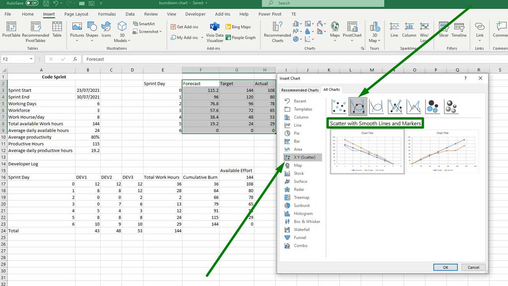
From “All Charts” select “X Y (Scatter)” and then select “Scatter with Smooth and Lines and Markers.”
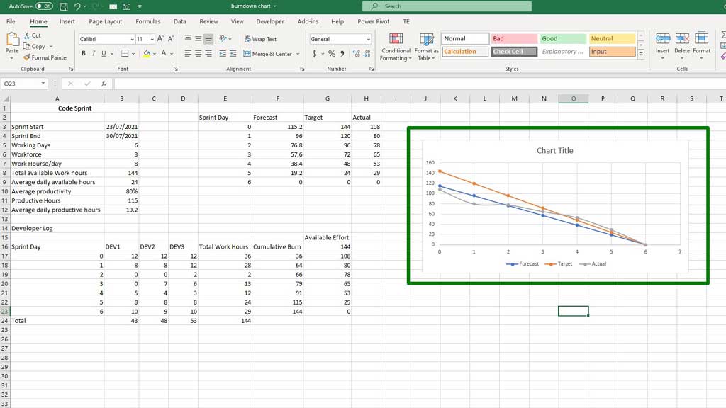
You will get a chart like this.
And voila, you have completed the steps of how to create a burndown chart in excel.
Now, let’s analyze the chart.
Analyzing the burndown chart in excel
The blue line depicts the forecast progress, the orange line depicts the target progress, and finally, the grey line depicts the actual progress.
The dots in the lines represent each sprint day.
If you hover your cursor over any dot, you will find all the information related to that day’s progress.
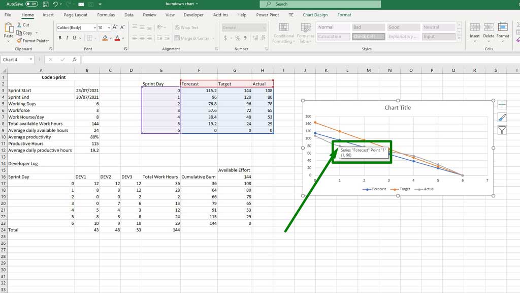
You can see that the actual progress is slow at first then it gains pace to complete the task. The pace exceeds the target to complete the task.
Conclusion
There you have it. It’s a simple 5 step method. Follow these steps and you will know how to create a burndown chart in excel. Now, being a manager is a little easier.

Hi there, I am Naimuz Saadat. I am an undergrad studying finance and banking. My academic and professional aspects have led me to revere Microsoft Excel. So, I am here to create a community that respects and loves Microsoft Excel. The community will be fun, helpful, and respectful and will nurture individuals into great excel enthusiasts.