How to Create a Stem and Leaf Plot in Excel?

Throughout my excel blogs, I have stressed that the use of excel in creating graphs and chart is extraordinary.

There are a lot of basic charts and graphs options built-in in excel itself. However, there are some charts and graphs used in statistics and other purposes that are not built-in but can be created in excel by tweaking the data.

For instance- the burndown chart, Venn diagram, supply and demand graph, etc.

One such graph is the Stem and Leaf diagram.

This particular graph does not have a built-in feature in excel. But it is possible to build it in excel.

So, let’s see how to create a stem and leaf plot in excel.

What is a Stem and Leaf Plot?

A stem and leaf plot is a diagram that maintains individual data points and summarizes them.

The plot splits a value into two parts. The first part is called the Stem and the last part is called the leaf. The stem is usually the first part or the first digit of a value and the last digit is the leaf.

The final digits (leaves) are sorted in a row in ascending order for every same stem.

How to Create a Stem and Leaf Plot in Excel?

To create a stem and leaf plot in excel, you first have to extract the stem and leaves from the value and then you can go on and create the plot.

So, let’s learn how to create a stem and leaf plot in excel.

Step#1 Sort the Values from Smallest to Largest

Suppose you have ages of different people. You have to create a stem and leaf plot of the ages.

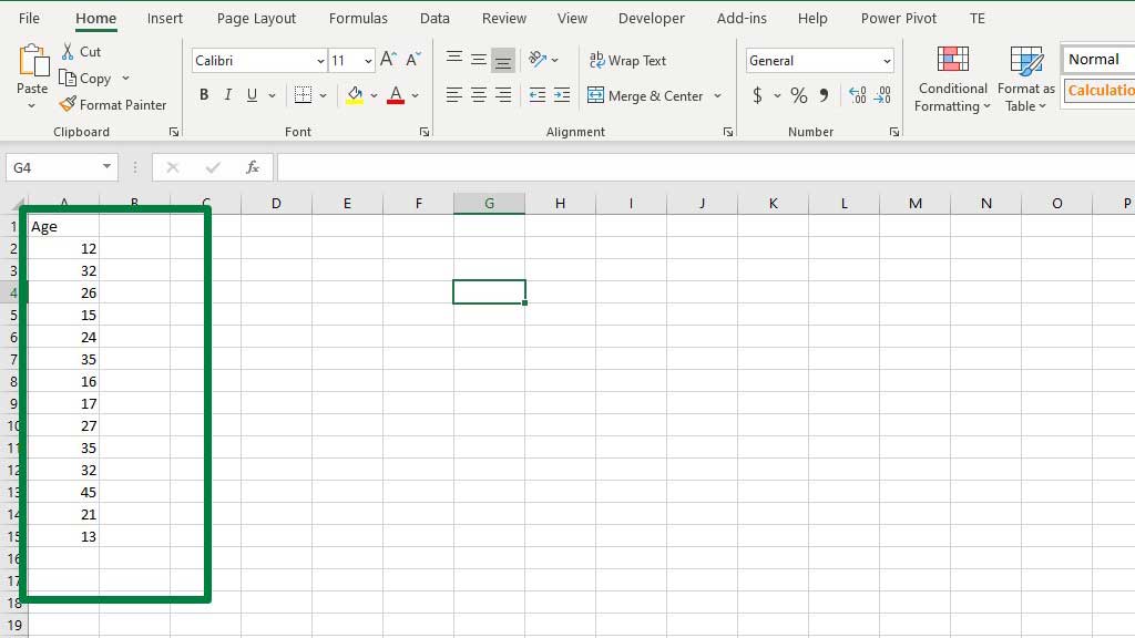
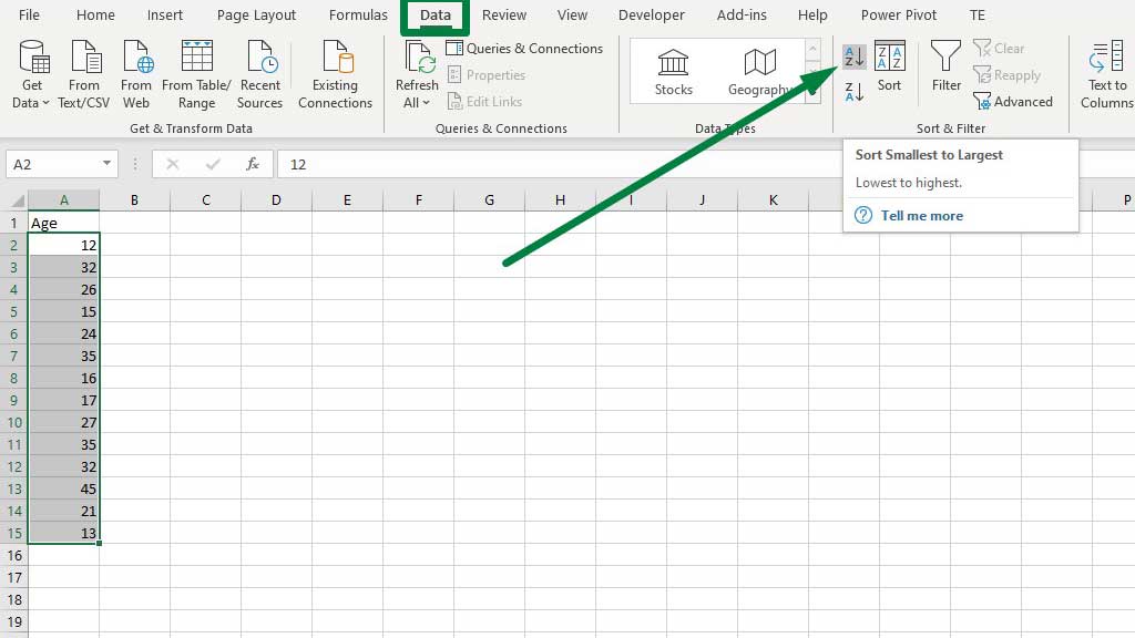
First, sort the values from smallest to largest.

Select the values and go to the Data ribbon and from the Sort & Filter tools select the smallest to the largest icon.

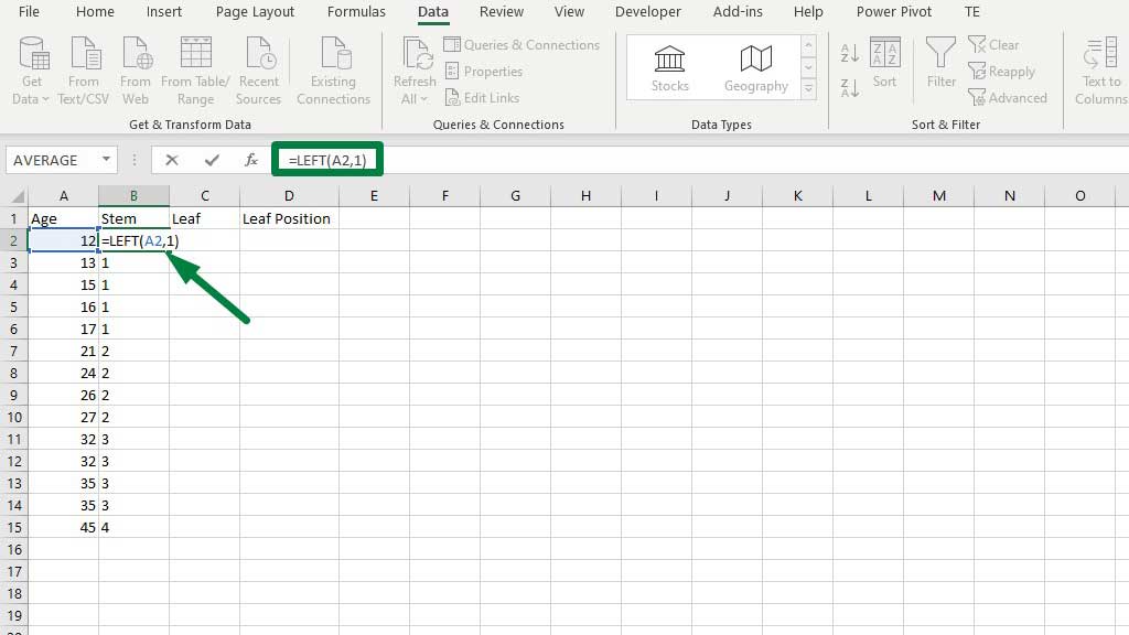
Step#2 Find the Stems and Leaves

To find stems and leaves you to need two formulas.

First, type the following formula to find the stems:

=LEFT(A2,1)

Now, type the following formula to find the leaves:

=RIGHT(A2,1)

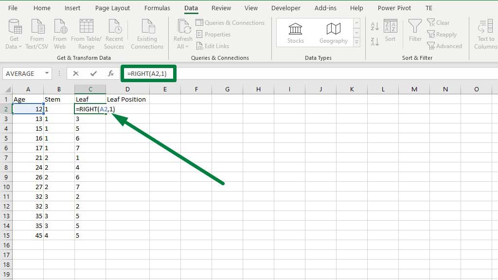
These two formulas essentially extract the digits you specify either from the right or the left. The first syntax is the value you want to extract the digit(s) from and in the last syntax you specify how many digits you want to extract.

Step#3 Determining the Leaves’ Positions

To find the positions of the leaves type the following formula:

=COUNTIF($B$2:B2,B2)

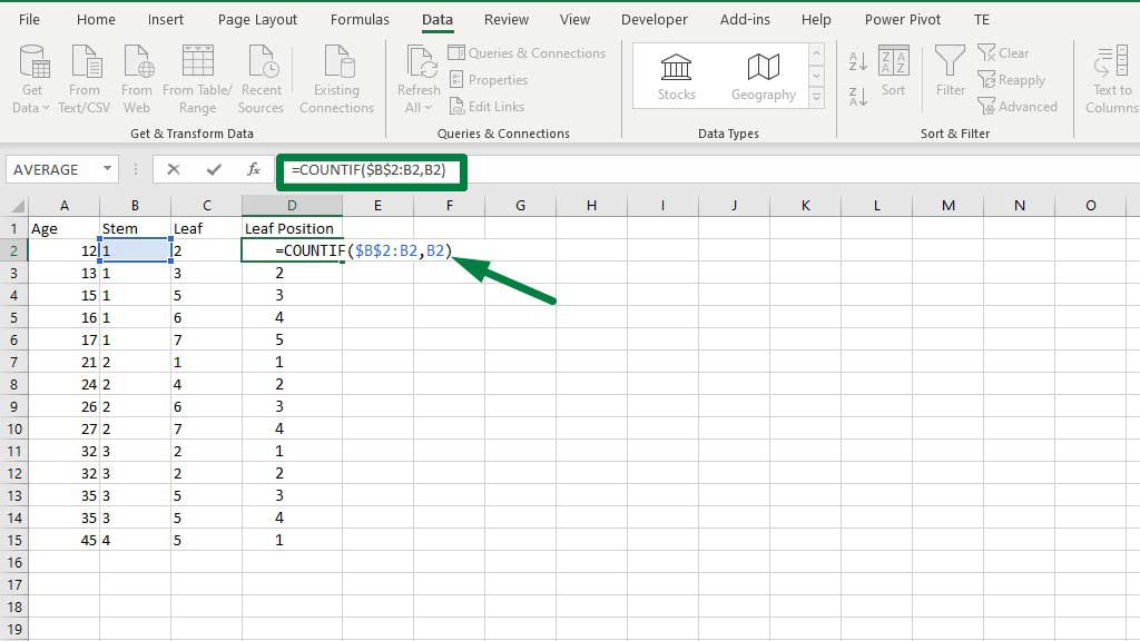
The formula essentially compares the stem values and finds duplicates. Then assigns the appropriate positions for the leaves.

Step#4 Create the Stem and Leaf Plot

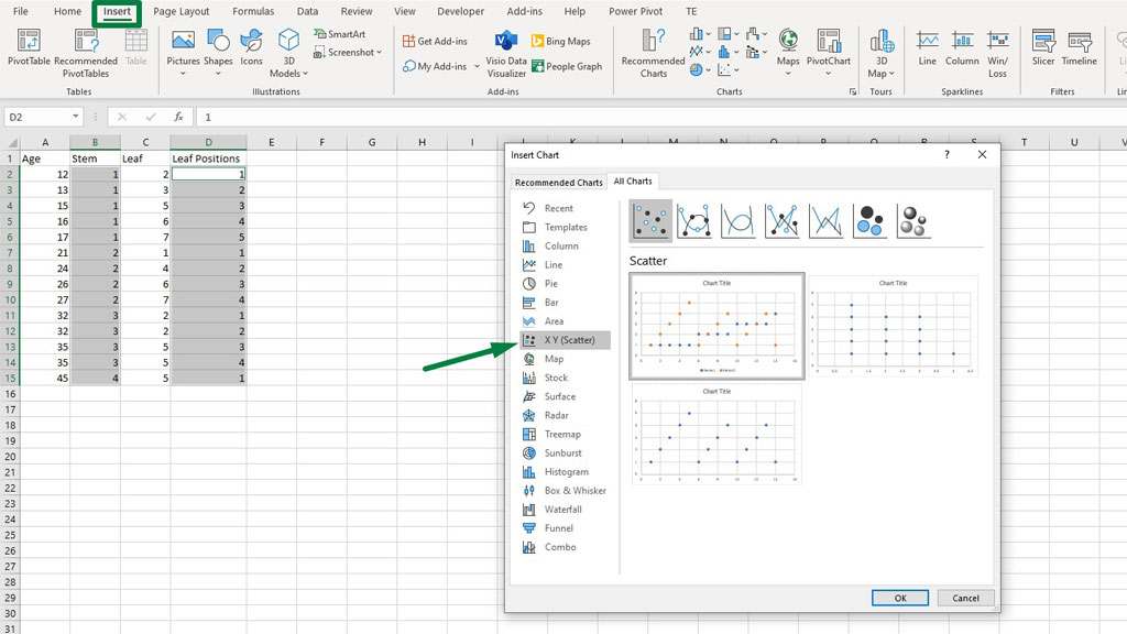
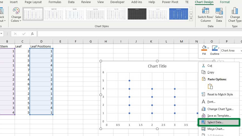
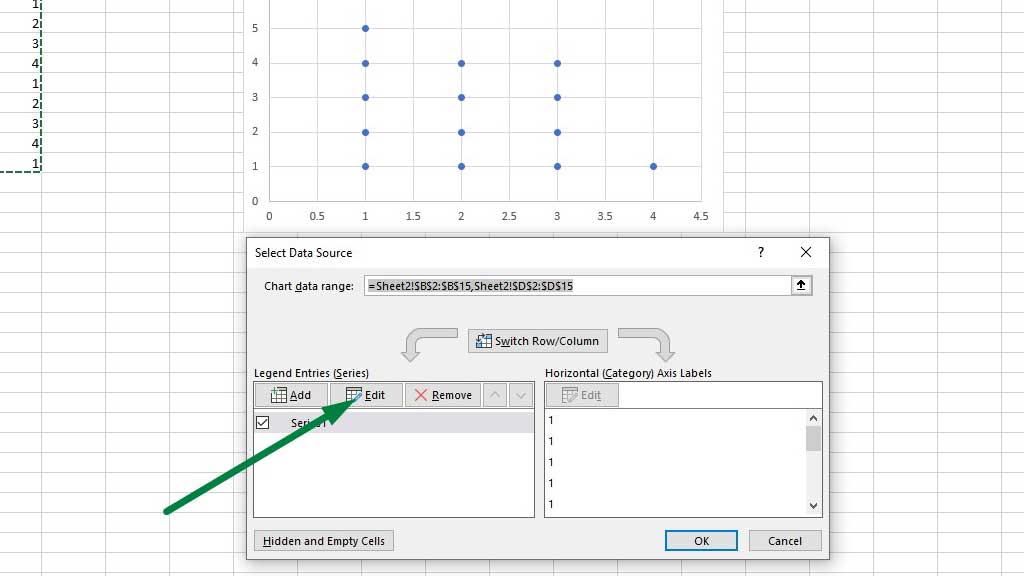
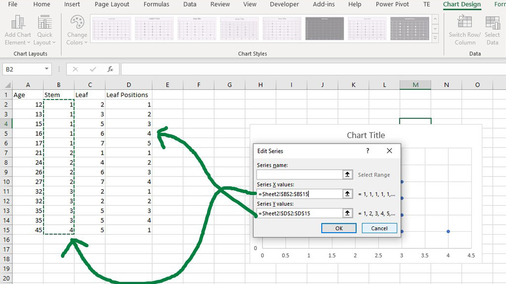
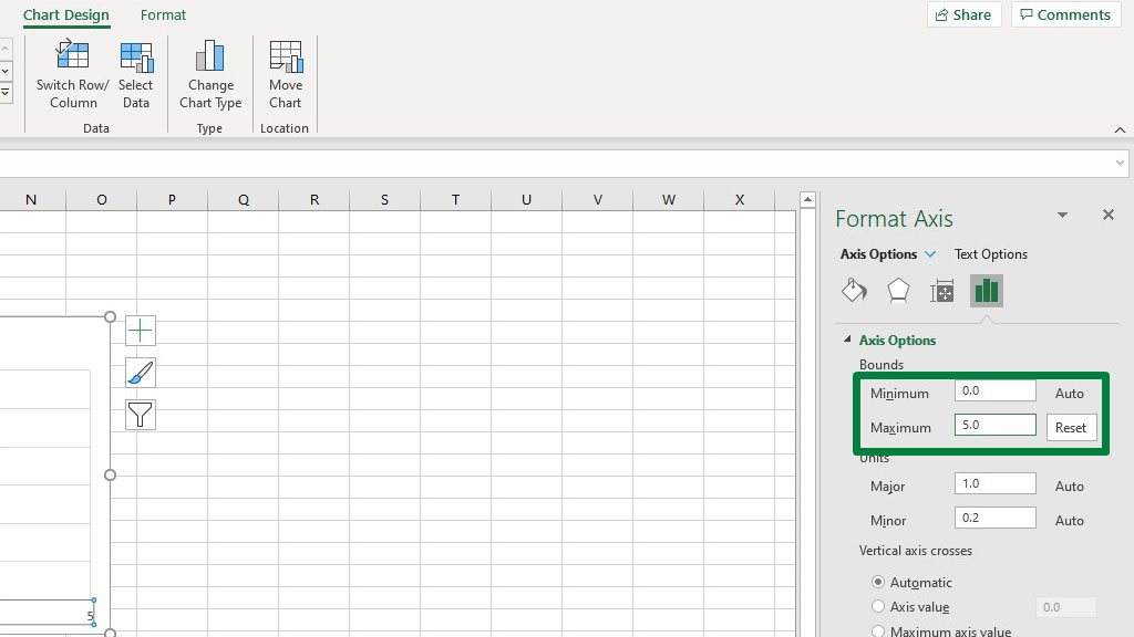
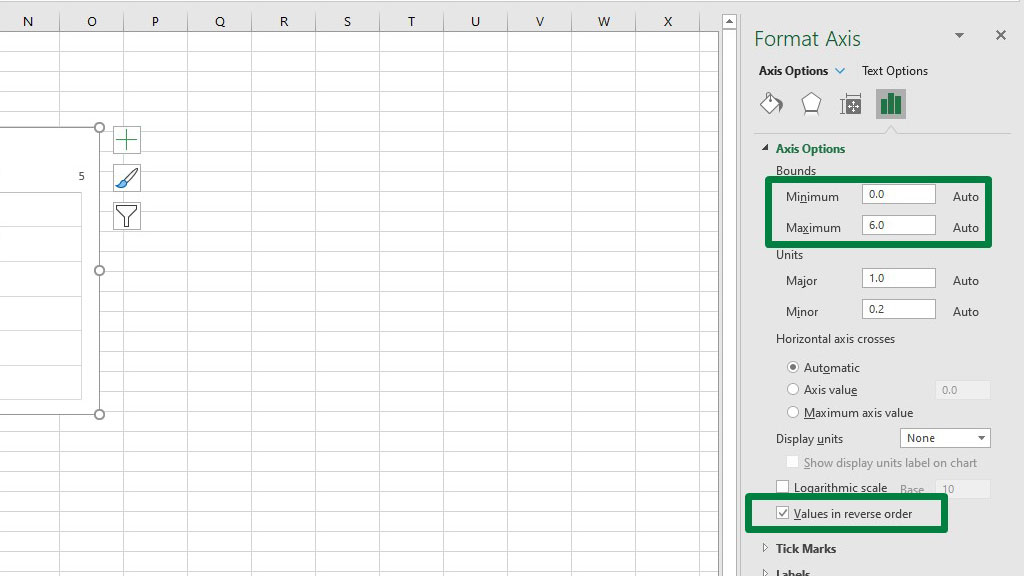
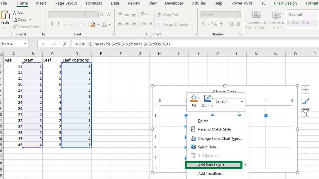
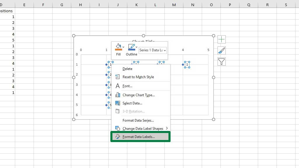
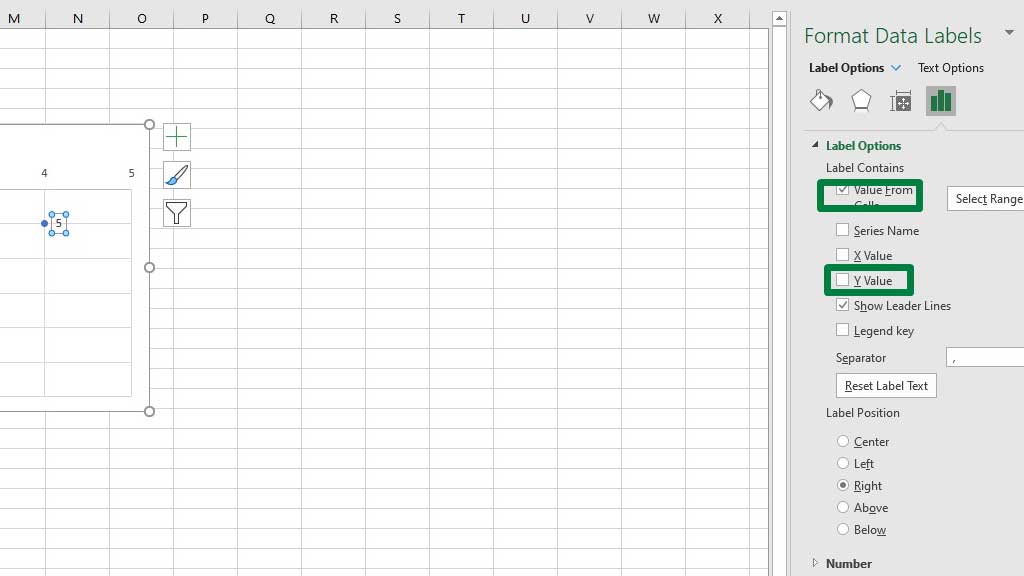
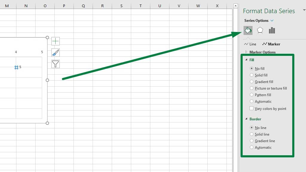
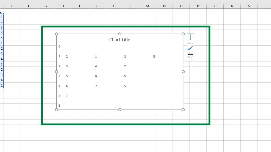
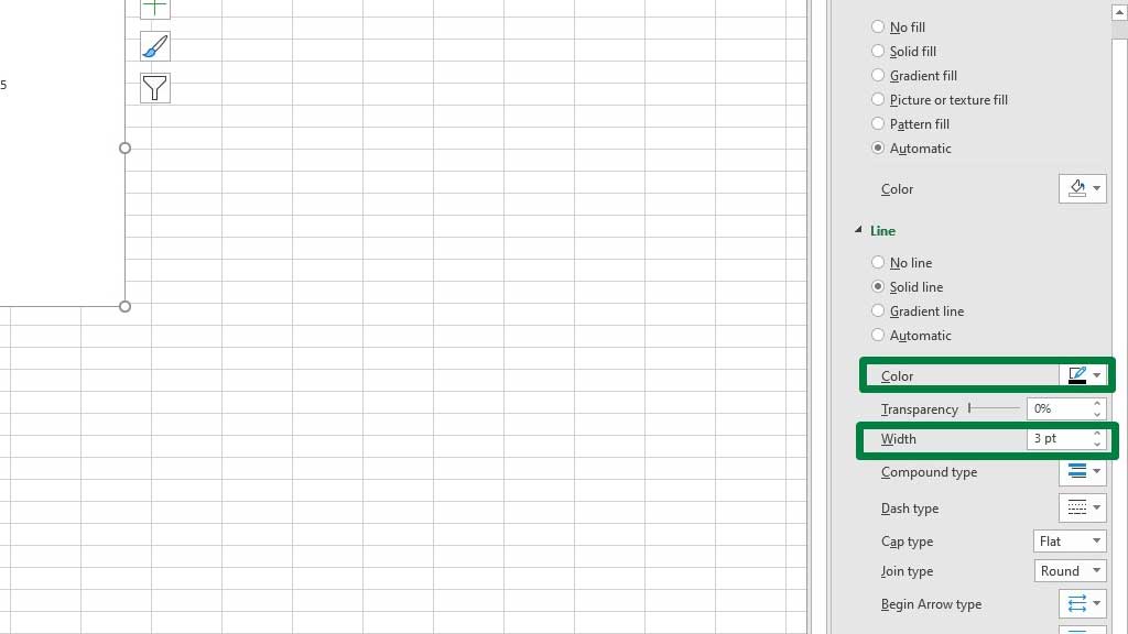
Now that the values have been sorted and extracted, you are ready to create the stem and Leaf plot.

First, select the stem column, and then holding the CTRL key select the leaf positions columns. Don’t select the label in any of the columns just select the values.

Now, from the Insert ribbon, go to Recommended Charts and select an X Y (Scatter).

Now, right-click on the graph and go to Select Data.

You will see a dialogue box pop up. From that box go to Edit.

Now, in the Series X values input the values of stems by selecting the stem column and Series y values input the values of leaf positions by selecting the leaf positions column.

Step#5 Formatting the Stem and Leaf Plot

Your stem and leaf plot is almost ready. You have to do some modifications to it to make it perfect.

First, double click the horizontal axis set the bounds to 0 and 5.

Now, double click the vertical axis and set the bounds to 0 and 6, and enable the Values in reverse order option.

Now, to add data labels. Select any of the markers or dots inside the graph and right-click and select Add Data Labels.

Now, to edit the data labels. Select any of the data labels inside the graph and right-click and select Format Data Labels.

Enable value from cells and select the Leaf column in the dialogue box. Uncheck the Y value.

Select the markers and go to marker options to select No fill and No line.

This will make the markers invisible.

Now delete the horizontal axis and all the grid lines to make the plot clean.

Finally, select the vertical axis, change the color to black, and set the width to 3 points.

There you go your stem and leaf plot in excel is ready.

Conclusion

Follow these steps and you can easily create a stem and leaf plot in excel. This is dynamic so you can add values as you wish and excel will update the chart automatically.

So, there you go now you know how to create a stem and leaf plot in excel.

Naimuz Saadat

Hi there, I am Naimuz Saadat. I am an undergrad studying finance and banking. My academic and professional aspects have led me to revere Microsoft Excel. So, I am here to create a community that respects and loves Microsoft Excel. The community will be fun, helpful, and respectful and will nurture individuals into great excel enthusiasts.