
While Microsoft Excel’s use can be versatile and most of its usage lies in business scenarios or data analysis. Using the software’s mathematical applications can make anyone’s life easier and faster.
One of the key aspects of Mathematics is Function. A function is best understood when it is graphed.
But we all know, graphing a function manually is very time-consuming, tedious, and sometimes difficult for multinomial functions.
Hence, the use of excel can make graphing of a function or an equation easy, fast, and visually appealing.
So, let’s jump into how to graph a function in Excel.
What is a Function?
First, let us define a function.
A function is a relationship between a dependent variable and an independent variable. A function measures the movement of a dependent variable with respect to the movement of an independent variable.
There are various functions in mathematics. In a previous blog, we showed how to graph a linear equation or function in excel.
Today, I am going to show three more functions to work within excel. You will know how to plot the graph in excel.
So, let’s start with how to graph a function in Excel.
How to Graph a Function in Excel?
The three functions we are going to work with here are quadratic function, trigonometric function, and logarithmic function.
Function#1 Graphing a Quadratic Function in Excel
A quadratic function is written in the form ax2+bx+c.
Here, a, b and c are constant.
So, let a be 3, b be 2 and c be 1.
So, the equation is 3×2 + 2x + 1.
And the function is y = 3 x2 + 2x + 1.
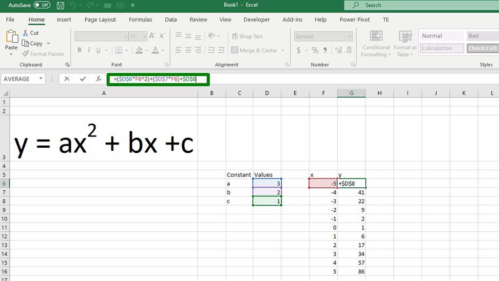
Now, let’s see how to input the values of x and get the corresponding values of y in Excel.
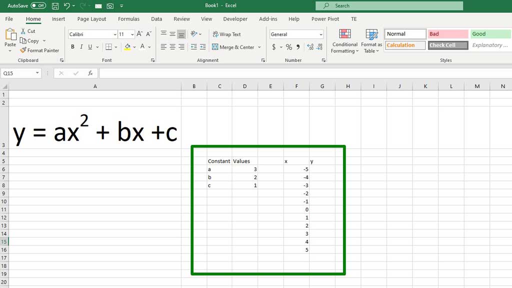
First, make a table like this in Excel to define the value of the constants and the independent variables (x).
Now, to get the values of y input the following formula:
=($D$6*F6^2)+($D$7*F6)+$D$8
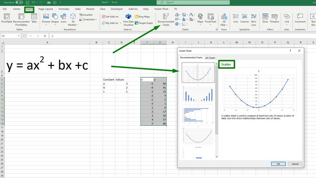
Now the values are ready to be plotted in a graph.
First select both the columns that contain x and y values, then from the “Insert” ribbon go to “Recommended Charts” select a scatter chart, and press ok.
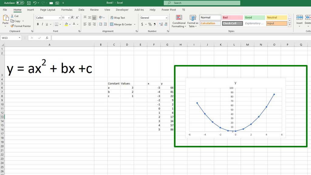
And there you have it. You have graphed a quadratic function in Excel.
Function#2 Graphing a Trigonometric Function in Excel
Let’s graph the SIN function in excel.
First, make a table like this.
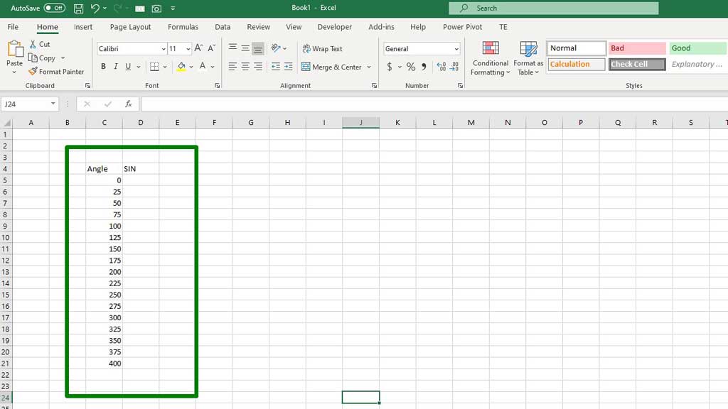
Inputting the angles can be tedious, so let me show you a trick.
Input the first angle 0 and then in the next cell type in the formula
=C5+25.
You can type any number instead of 25, depending on your preference of the difference you want to keep between two angles.
Then drag your fill handle down until you reach your preferred last angle for the function.
Now, input the formula to get the values for the SIN function in excel.
=SIN(RADIANS(C5))
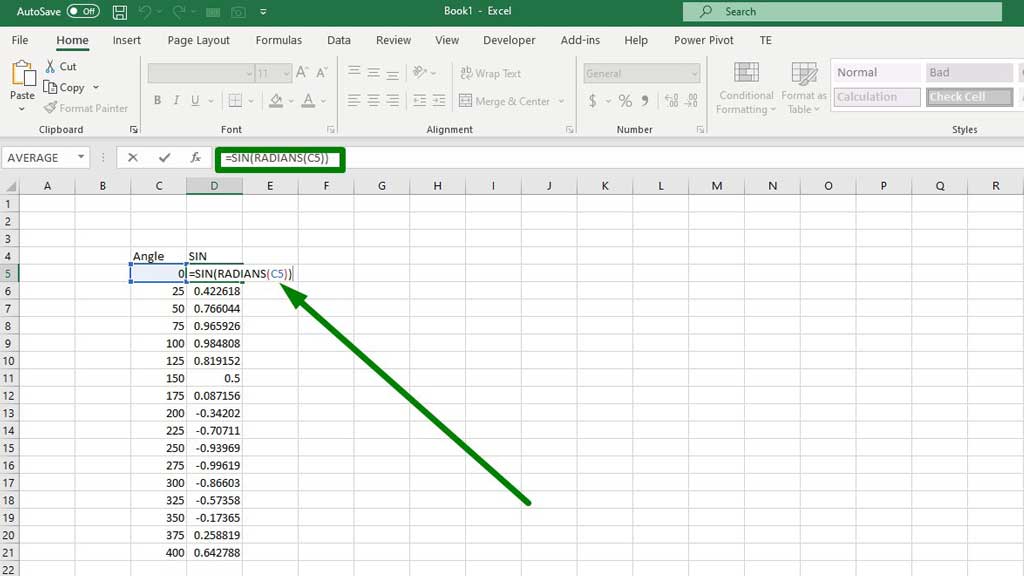
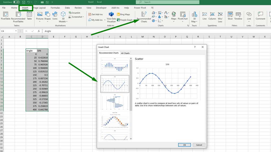
Now the values are ready to be plotted in a graph.
First select both the columns that contain the angles and the SIN values, then from the “Insert” ribbon go to “Recommended Charts” select a scatter chart, and press ok.
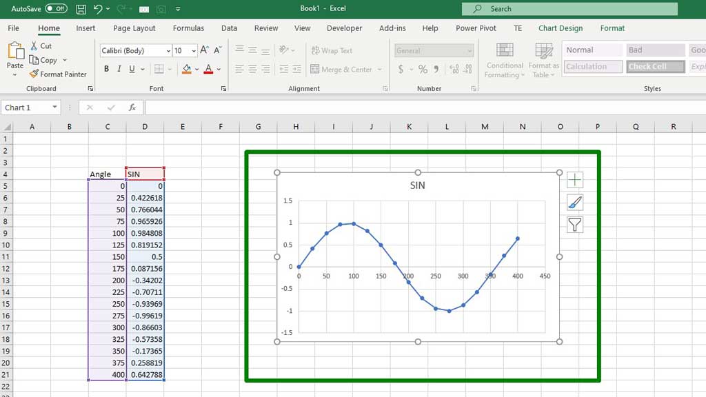
And there you have it. You have graphed a trigonometric function in Excel.
Function#3 Graphing a Logarithmic Function in Excel
Let’s graph a logarithmic function in excel that has a base of 10.
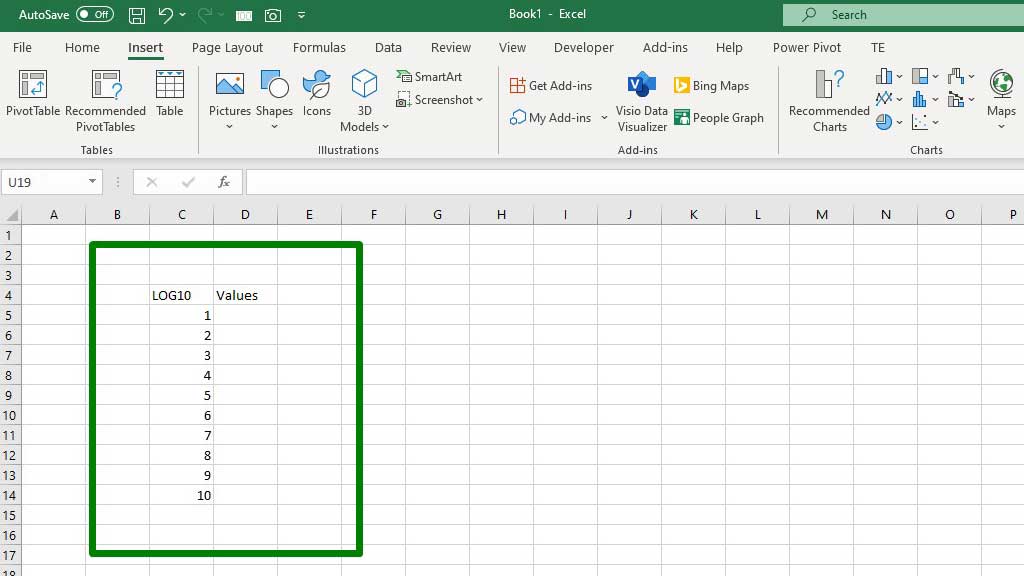
First, like all the other functions, make this table that contains the values.
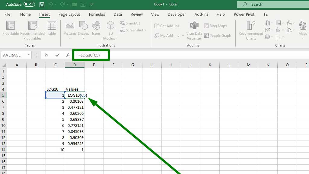
Then input the formula to get the corresponding values
=LOG10(C5)
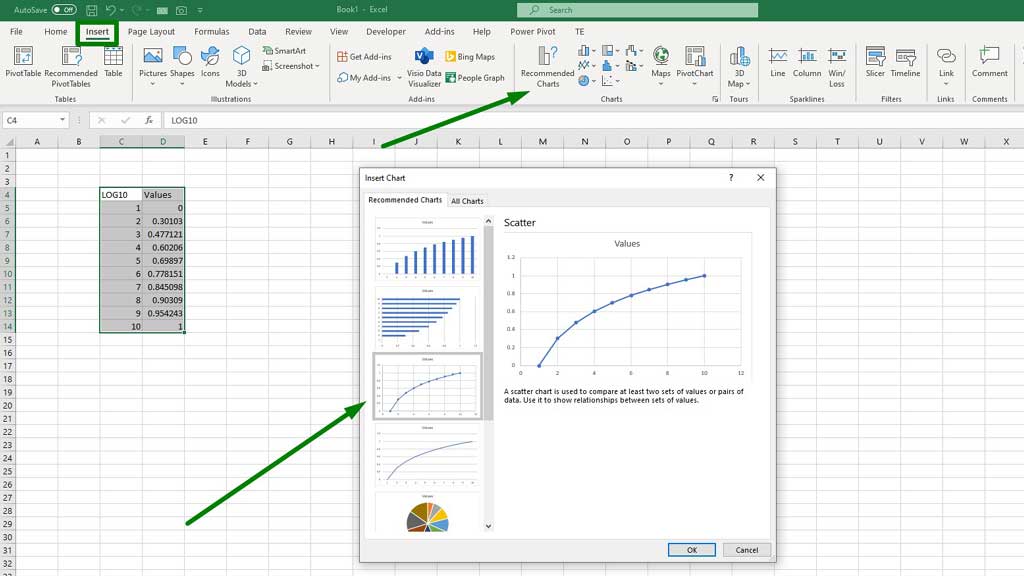
Now the values are ready to be plotted in a graph.
First select both the columns, then from the “Insert” ribbon go to “Recommended Charts” select a scatter chart, and press ok.
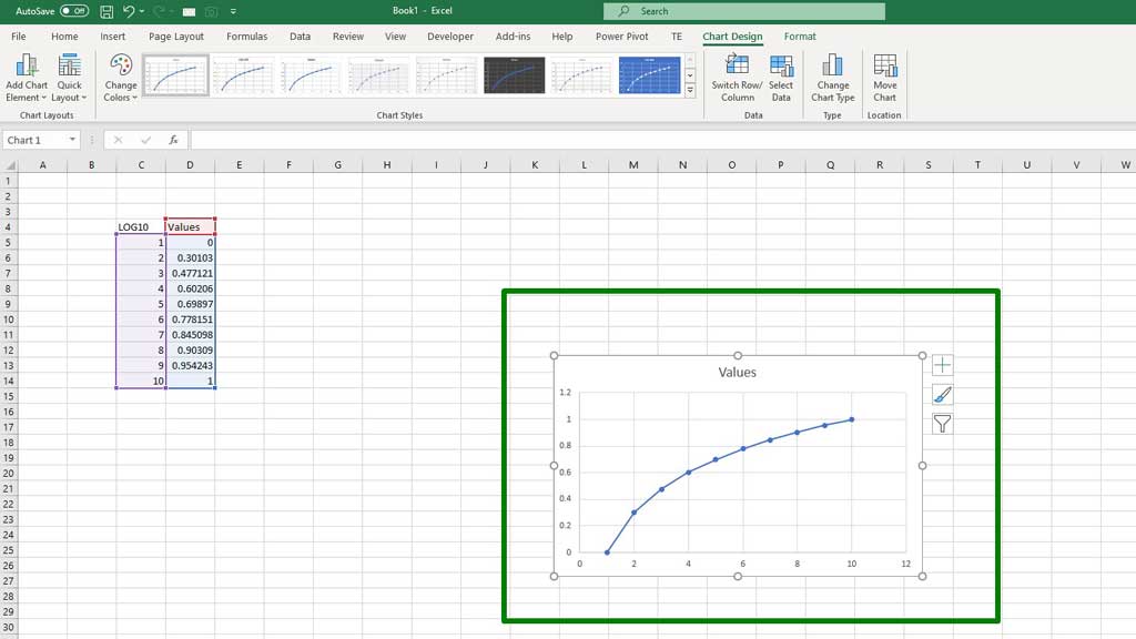
There you go, the graph for the logarithmic function in excel is ready.
To make the graph more visually appealing and easy to understand, you can add data labels to the graph.
Select a graph, then go “Chart Design” ribbon and go to “Add Chart Elements” and go to “Data Labels” to select your preferred form of a label.
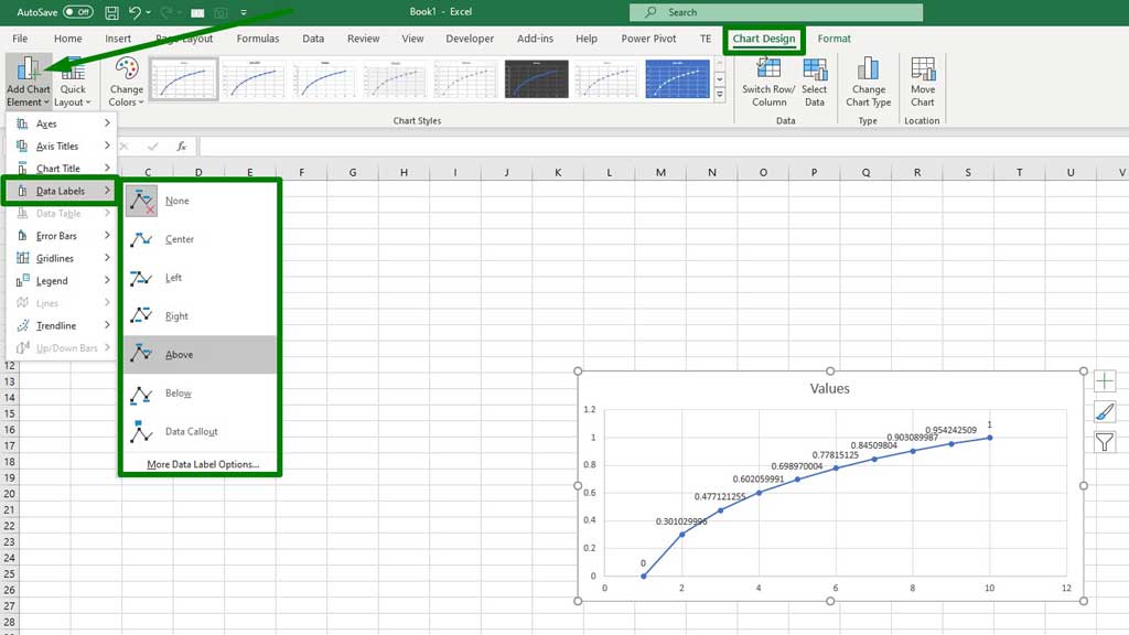
You can also change the colors or other layout options from this ribbon as you wish.
Conclusion
Today you have learned a valuable lesson of graphing functions. Using these steps and methods you can graph any function or equation in excel.
So, from now on you can be more precise in mathematics or you can help your friends by showing them how to graph a function in excel.

Hi there, I am Naimuz Saadat. I am an undergrad studying finance and banking. My academic and professional aspects have led me to revere Microsoft Excel. So, I am here to create a community that respects and loves Microsoft Excel. The community will be fun, helpful, and respectful and will nurture individuals into great excel enthusiasts.