How to Make Negative Numbers Red in Excel?

Working with numbers, analyzing data, and visualizing the results to have a significant impact on a business or project is ever so easy to do in excel.

Excel has multiple features and formulas that make numbers and data speak, maybe not in a literal sense but excel makes them lively enough to have an impact on practicality.

Such impactful features include conditional formatting and custom number formatting.

These features are very helpful when identifying numbers that belong to a range, numbers that are greater or less than other numbers, positive and negative numbers, etc.

So, today we are going to use these features and learn how to make negative numbers red in excel.

How to make negative numbers red in excel?

Analysts work with heaps of numbers and data in excel. That’s why distinguishing them for different purposes becomes a crucial task to visualize impactful results.

That’s why formatting, highlighting, etc. is a necessary practice while working n excel.

For example, you run a business and keep track of all transactions in business. To keep track of the losses and the outgoing cashflows you decide to make the numbers red.

To do that you can use two features in excel, conditional formatting, and the other custom number format.

So, let’s see how to make negative numbers red in excel.

Method#1 Making negative numbers red in excel using the conditional formatting tool

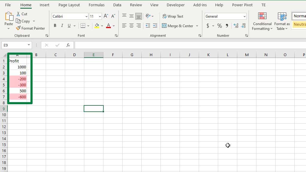
In the picture, you can see that there are several numbers with positive or negative values. When the numbers keep on piling it will be hard to distinguish among them.

So, let’s see if we can make the negative numbers red.

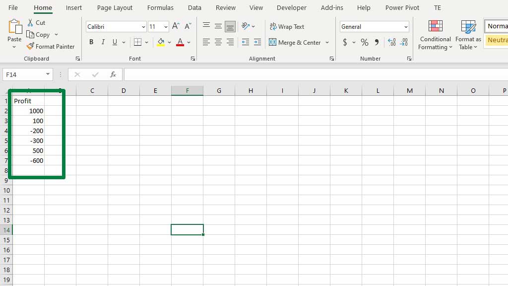
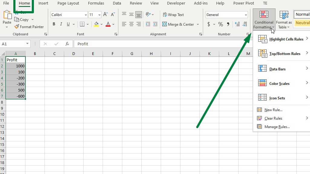
First, select the numbers and then go to Conditional Formatting from the Home ribbon.

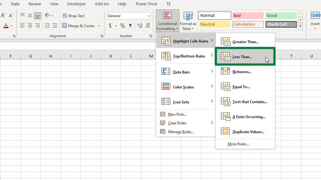
Then from the Highlight Cell Rules select Less Than.

Now, as all negative numbers are less than 0, type 0 in the less than box and choose a red color. There are several red color options (red border, red text, light red fill, etc.) but I have chosen the light red fill with dark red text.

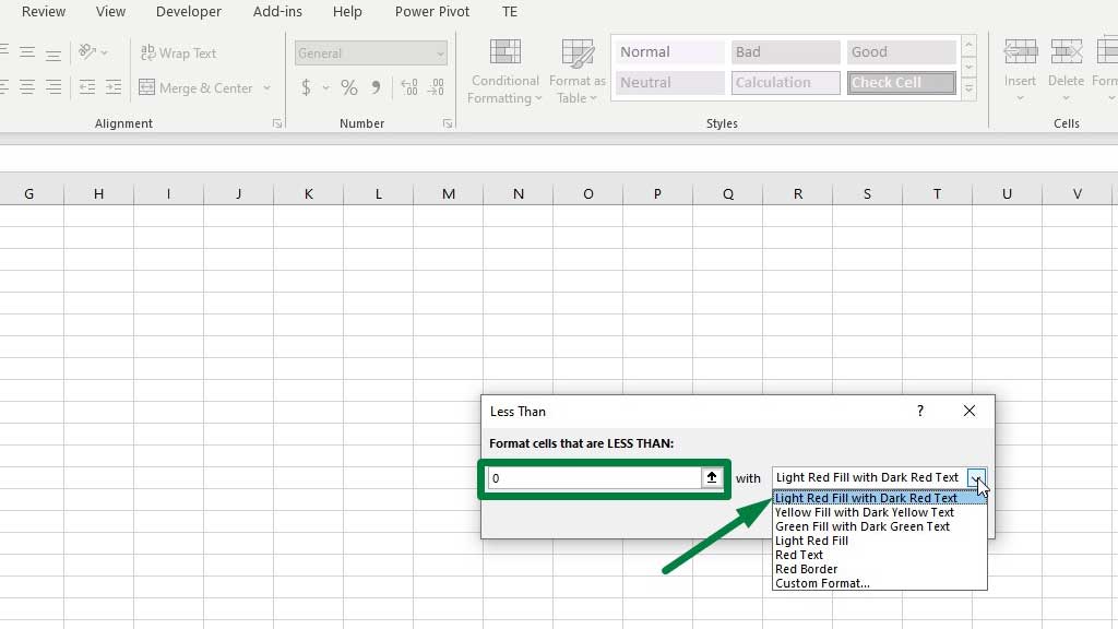
You will already see that all the negative numbers have been highlighted in red.

You can also choose a custom color format. You can also highlight or format numbers that are greater than other numbers, top or bottom numbers, between numbers, etc. with the same principle.

So, this makes the conditional formatting tool a very powerful feature in excel.

Method#2 Making negative numbers red in excel using the custom number format

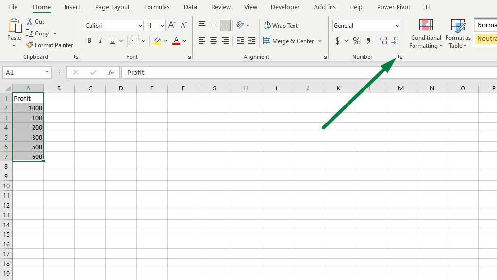
Select the numbers then go to the Number Format or use the shortcut CTRL+1.

From the number formats select the red numbers. You can set decimals places as well.

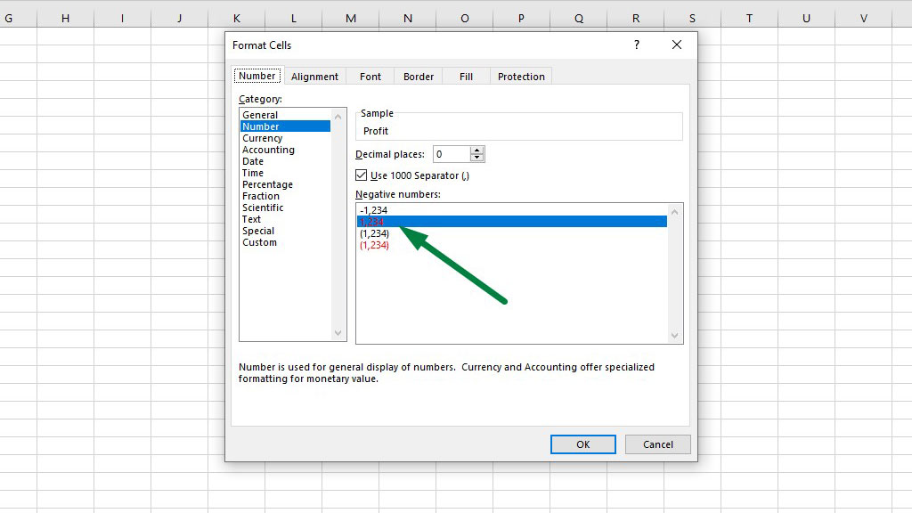
If you go to the custom number format you will see more formats that let you make the negative numbers red. You can also choose if you want the negative numbers inside a bracket or not.

Usually, accountants use brackets and red colors to denote the negative numbers.

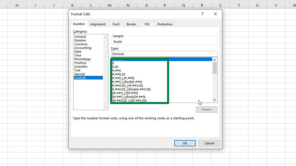
There are different codes for the formats. The hashtags (#) represent numbers. The commas are a thousand separators, dots are the decimals, brackets will only encompass the negative numbers.

So, there you go now you know how to make negative numbers red in excel.

Conclusion

There are numerous formatting options in excel that let you format, highlight and display numbers as per your requirement.

In this article, only a small portion of the formatting techniques possible in excel has been shown.

As now you know how to make the negative numbers in excel and use the conditional formatting, practice and explore, and soon you will be able to do more than just highlighting negative numbers.