
A sales meeting is going on. The manager is sitting with the 10 salesmen he manages. He has made a chart for the past 5 years to review profits generated by the salesmen.
The agenda of the meeting is to review the performance. But only displaying numbers is not visually appealing. There are 10 salesmen, so creating individual charts or graphs is also not feasible.
So, what can the manager do?
Fear not, Excel is here to the rescue. The manager can create a sparkline for each of the salesmen and make the figures look visually appealing and more understandable.
So, without any further ado, let’s look at how to create a sparkline in Excel.
What is Sparkline?
Sparklines are essentially graphs or charts, smaller in size, that are created inside a cell.
Sparklines are created to show variations in data or trends.
It is a great tool to make data visually appealing and they help to identify patterns in a more limited setting.
However, functionalities related to a sparkline are not as versatile as a graph or chart in excel.
How to Create a Sparkline in Excel?
Now, let’s look at the functionalities that come with creating a sparkline in excel.
Creating a Sparkline in Excel
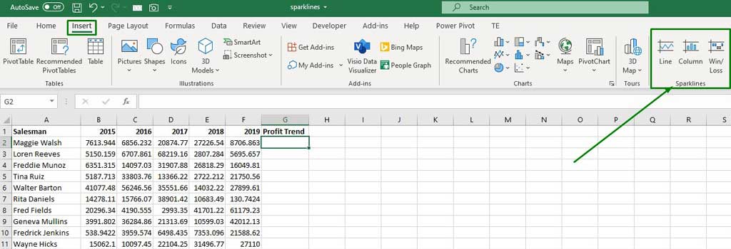
First, select the cell you want to create the sparkline in. Then go to the “Insert” Ribbon and select your preferred sparkline.
A dialogue box will appear. You will need to select the data range for which you want to create the sparkline.
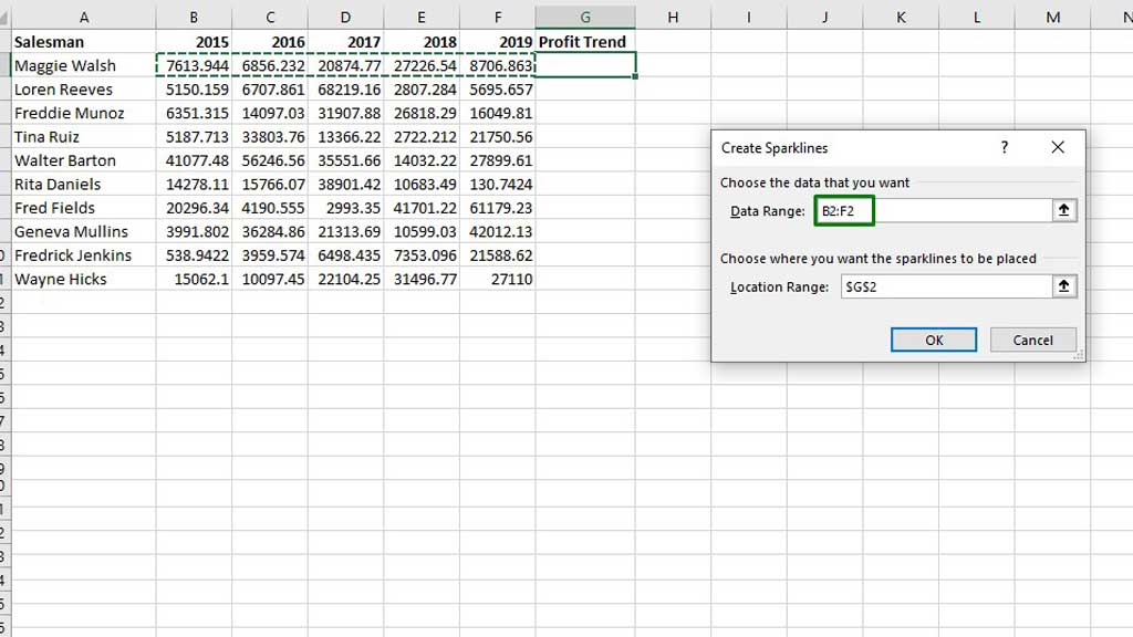
Select the data range for the sparkline and click ok.
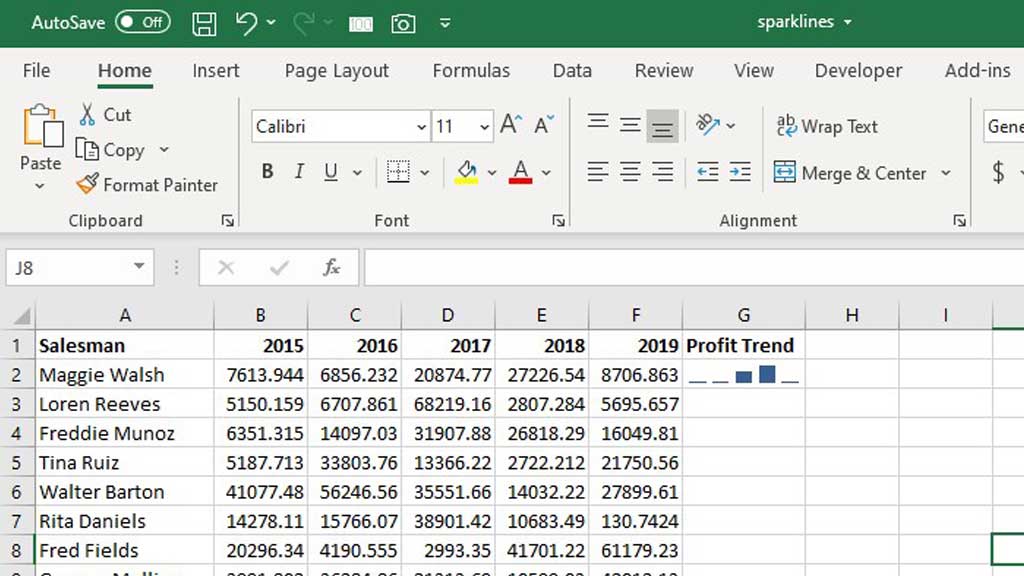
Now, select the cell you created the trendline in and move your cursor to the bottom right corner of the cell to bring out the fill handle. Now, drag your fill handle down to create sparklines for the other profit trends as well.
Voila, you have successfully created sparklines in excel.
Highlight Important Points of Data
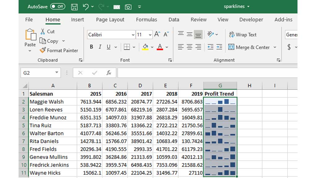
Now, the manager wants to highlight the highest profits for each salesman. To do that, select a sparkline and go to the “Sparkline” ribbon and select “High Point.”
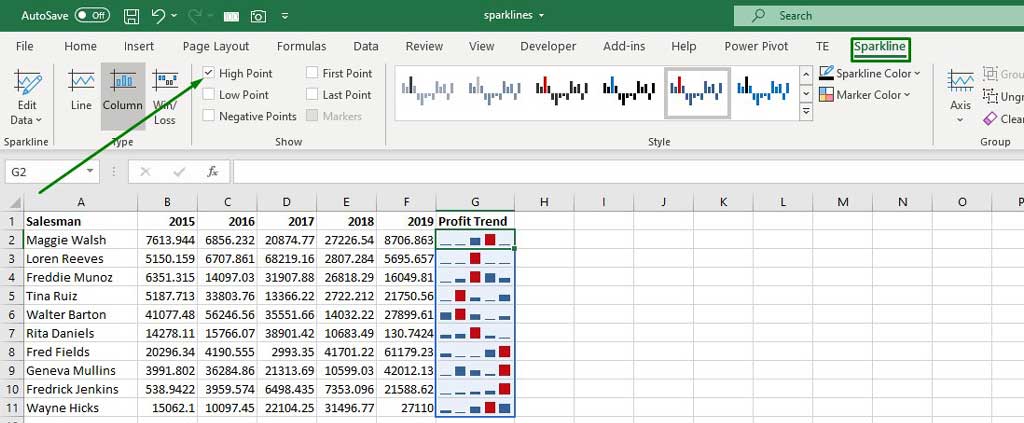
This will highlight all the highest profits.
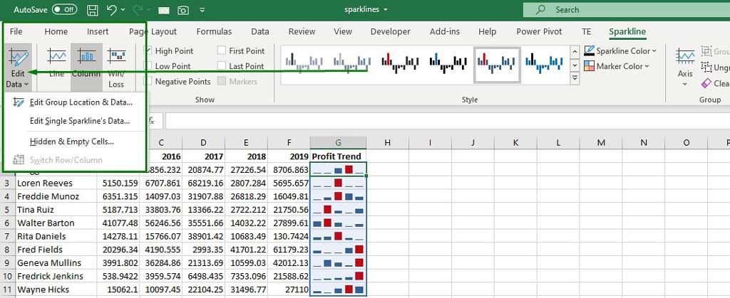
You can also edit your data from the “Edit Data” Option.
Important features of Sparkline
- You can edit your dataset and the sparklines will automatically get updated.
- increase the height or width of the cell to adjust the size of a sparkline.
- You can enter any text even if there is a sparkline in a cell.
- The colors or type of the sparklines can also be changed or edited.
Conclusion
There you have it. It is very simple to create a sparkline in excel. Follow the steps of how to create a sparkline in excel and stand out in presentations.

Hi there, I am Naimuz Saadat. I am an undergrad studying finance and banking. My academic and professional aspects have led me to revere Microsoft Excel. So, I am here to create a community that respects and loves Microsoft Excel. The community will be fun, helpful, and respectful and will nurture individuals into great excel enthusiasts.